Consuming a Query in Excel PowerView in Microsoft Dynamics NAV 2013 R2

First things first, lets clear what we are going to discuss here today. We are going to configure Excel's PowerView feature to visually demonstrate the Navision tables data. Power View is an interactive data exploration, visualization, and presentation experience that encourages intuitive ad-hoc reporting in Excel. This is a feature of Microsoft Excel 2013.

Prerequisites - Microsoft Excel 2013, Microsoft Silverlight.

Now, to demonstrate the feature we are going to visually represent the Profit by Country by using the data from Customer table. 

We are going to demonstrate it in just 3 very easy steps as follows:

Step 1 : Create a Query and Publish it as an OData WebService

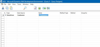
• Open the Development Environment and Create a New Query Object.

• Define a Data Item. (i.e. you can use Customer table)

• Open the Field Menu and Select the Field you want to include in the Query.

• Save the Query.
• Run the Query to verify the correctness of the Query.
• Now from the RTC search for 'Web Services' and open it, a page opens.
• Click on New to create a new Web Service.
• Select 'Query' as Object Type, enter the Object ID, type in the Service Name and then Click on Publish to Publish the Web Service.

• Copy the OData URL from the Web Services Page and paste it on Internet Explorer to check whether the Web Service is working or not.

Step 2 : Create an Excel Workbook and Insert a Powersheet into it.

• Go to Insert and Click on PowerView to insert a PowerView Sheet.
• When you Create a PowerView sheet for the first time, Excel asks you to enable the PowerView add-in. Click on Enable.

Step 3 : Establish a Data Connection from Excel directly to the new OData URL and visualize the data in the PowerView.

• In the Excel, Click on PowerPivot and then Click on Manage.
• Inside the PowerPivot, Click on From Data Service and then From OData Feed.

• In the Pop-up window, Paste the Copied OData URL and then Click Next then Click on Finish.

• Now close the PowerPivot and Refresh the PowerView Sheet. The CustomerSales is shown as Power View fields in the Right Menu.
• Drag the Country Region Code field on the main page. As we want to see it visually so we select the Map option in the Design Menu on Top Bar.

Now the Fun part 

There is a lot to interact in the PowerView sheet that you have created. Play with the fields in the Customer Sales. 

• Drag the Profit (LCY) to show the data in the Map with the Profit by the Countries.
• You can also add colour to the Name of the Customer by dragging the Name field to the Colour box at the bottom.
• You can add any field as a filter by dragging the field to the filter area. For example, you can filter the data by the Salesperson Code by selecting the particular Salesperson from the Filters menu. 

I hope you are caught up with the whole process. Write your comments below if you are facing any problem with the configuration. Watch the whole process in the video below to understand the concept more clearly about Excel Powerview and its use in Microsoft Dynamics NAV 2013 R2 and also Subscribe to our Youtube channel.